Underscoring With Deep Learning

This post is a very condensed overview of my master’s thesis. In short, it was an attempt to model the relationship between underscoring and films by using deep learning.

The motivation for this project was to improve the searchability of production music libraries, especially those including pop songs, which are often available for commercial licensing but have tags applied with the average consumer in mind, not music supervisors. Automated annotation and better search for production music could streamline a very time- and labor-intensive process and increase the chance that tracks by lesser known artists get a fair hearing by the right people.

Compiling Training and Testing Data

Neural networks need a lot of well-labeled data, and the more complex the network, the more data you need. The data preparation process has at least two steps:

• Collect raw data for input

• Optional: Compress data through feature extraction

• Link input data to consistent and accurate ground-truth labels

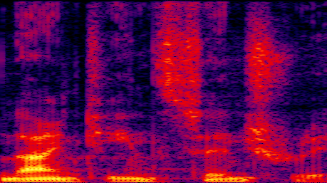
The final input data were arrays of 100 concatenated frames of the first 40 Mel-Frequency Cepstral Coefficients, comprising about 10 seconds of audio each. The use of a feature vector is not strictly necessary for a deep network: given enough training, a network will learn intermediate features (which can be superior to ‘engineered’ features like MFCCs) directly from spectrograms. However, spectrograms take up memory equivalent to uncompressed PCM audio, and when handling sets of data that represent hundreds of hours of audio they quickly become completely unwieldy.

Using MFCCs allows compression on the order of 90% by keeping a few coefficients that describe the rough shape of the spectrum. In short, MFCCs generate a ‘filter-excitation’ model of the signal, and discard the ‘excitation’ component. The audio cannot be satisfactorily reconstructed from the MFCCs, but they are extremely effective for models dependent on timbre and rhythm rather than pitch.

Below is a sample of what an audio signal reconstructed from MFCCs sounds like, crossfaded with the original signal. Since the MFCC algorithm discards the upper cepstral coefficients that represent the ‘excitation’ component, wide-band noise must be used to excite the filter, creating a rough, whispery effect.

Each tile is linked to one or more genre tags drawn from the Internet Movie Database. When dealing with multi-labeled input, there are two ways of arranging the data, depending on your network architecture:

• Link each input to a binary vector of length K, where K is the total number of possible labels.

• Duplicate the input for each label, using the duplicates to train independent binary classifiers, and aggregate the predictions of the ensemble.

I chose the second route, allowing for a more thorough use of the data at the expense of increased training time.

The ground-truth labels have some interesting characteristics, with a high degree of overlap between some labels and none between others. Some label sets are very large, especially “Drama”. In the interactive plot below, note how some labels are nearly completely subsets of “Drama”.

This was probably a clue that the “Drama” tag carried almost no information, but I couldn’t set it aside without losing a ton of soundtracks that were only tagged as Dramas, so I went ahead and included them anyway.

Deep Learning and ConvNets

There are a ton of excellent tutorials on the basic inner workings of neurals networks, so I’ll try not to retread to much here. I’d like to focus on convolutional networks and how the same properties that give CNNs the ability to recognize rotated, flipped, and scaled images is useful for audio, too.

One of the biggest problems with using a fully-connected network for audio analysis is that it cannot encode any time-dependent information. Even if you try to use concatenated frames as feature ‘tiles’, any connections between adjacent pixels are destroyed in the process of unraveling the tile into an input vector. At best, long-term features could be generated by pooling across frames, but no sequential information is preserved.

Convolution networks work around this by changing the way that the neurons sum their inputs. Instead of summing a weighted vector from the entire input layer, the neuron in a convolutional network only ‘looks’ at a small region of the input with a correspondingly small set of weights (the kernel), and encodes a ‘stack’ of activations for each kernel position. In between layers, data is down-sampled (‘max-pooled’), so each successive layer ‘sees’ a larger portion of the image and detects more complex combinations of earlier kernel activations.

A convolutional layer is agnostic to transformations of the data, so neurons activate in the presence of a feature independent of its precise position and orientation. At the same time, spatial relationships between intermediate features combine in higher level features, encoding sequences through frames and across cepstral bins.

Implementation in Python

The convolutional networks were created with Theano, an open-source machine learning library for Python, with most of the scripting done with the Lasagne and Nolearn wrappers for Theano. My implementation was heavily informed by Daniel Nouri’s excellent tutorial on building an ensemble of specialist deep networks.

First we define our network hyperparameters for each of 10 network instances. The each network has 8 layers total: 1 input layer, 4 convolutional layers, 2 fully-connected layers, and a single neuron on the output layer. The output neuron gives a value in between 0 and 1 which will be used as a rough confidence metric for the presence of a genre tag.

epochs = 1000
dropout1 = .1
dropout2 = .2
dropout3 = .3
dropout4 = .4
dropout5 = .5
c1 = 32
c2 = 64
c3 = 128
c4 = 256
h5 = 50
h6 = 50
batch = 1200
rate = .01
momentum = .9

Then we create a neural network instance with a single call to nolearn.Lasagne.NeuralNet, using our previously defined hyperparameters. There is a dropout layer in between each layer to regularize the neurons and prevent overfitting, and a simple EarlyStopping function polls the validation error after each epoch and breaks out of the training loop after 30 consecutive increases in validation error. regression = True so that we can directly look at the activation of the output neuron.

CNN = NeuralNet(

	layers = 
	[ 

    ('input', layers.InputLayer),
    
    ('conv1', Conv2DLayer),
    ('pool1', MaxPool2DLayer),
    ('dropout1', layers.DropoutLayer),
    
    ('conv2', Conv2DLayer),
    ('pool2', MaxPool2DLayer),
    ('dropout2', layers.DropoutLayer),
    
    ('conv3', Conv2DLayer),
    ('pool3', MaxPool2DLayer),
    ('dropout3', layers.DropoutLayer),
    
    ('conv4', Conv2DLayer),
    ('pool4', MaxPool2DLayer),
    ('dropout4', layers.DropoutLayer),
    
    ('hidden5', layers.DenseLayer),
    ('dropout5', layers.DropoutLayer),
    
    ('hidden6', layers.DenseLayer),
    
    ('output', layers.DenseLayer),
    
    ],

'''
Hyper-parameters 
'''

	input_shape=(None, 1, 40, 100),
	conv1_num_filters = c1, conv1_filter_size = (5, 5), pool1_pool_size = (2, 2),
	dropout1_p = dropout1,
	conv2_num_filters = c2, conv2_filter_size = (4, 4), pool2_pool_size = (2, 2),
	dropout2_p = dropout2,
	conv3_num_filters = c3, conv3_filter_size = (2, 2), pool3_pool_size = (2, 2),
	dropout3_p = dropout3,
	conv4_num_filters = c4, conv4_filter_size = (2, 2), pool4_pool_size = (2, 2),
	dropout4_p = dropout4,
	hidden5_num_units = h5,
	dropout5_p = dropout5, 
	hidden6_num_units = h6,
	output_num_units = 1, 
	output_nonlinearity = sigmoid,

	update = nesterov_momentum,
	update_learning_rate = theano.shared(float32(rate)),
	update_momentum = theano.shared(float32(momentum),
	on_epoch_finished = [
	    AdjustVariable('update_learning_rate', start = 0.01, stop = 0.0001),
	    AdjustVariable('update_momentum', start = 0.9, stop = 0.999),
	    EarlyStopping(patience = 30),
	    ],

	batch_iterator_train = BatchIterator(batch_size = batch),
	regression = True, 
	max_epochs = epochs,  
	verbose = 1
)

After a long night of running the training loop on each network, the average validation error came down to 0.22. Unsurprisingly, this was about 10 times smaller than the validation error on a single multi-class network. I won’t bore you with all the metrics for evaluating multiple tagging algorithms, but if you’re interested they’re covered in the text of my thesis.

Making Predictions

Finally, we can actually see the network make predictions about the related film genres of the held-out test tracks. The plot below automatically cycles through the 196 tracks in the test set, showing the normalized predictions by bar length and the actual ground-truth labels with bright green bars. Simply put, if the green bars are longer, that’s a more accurate prediction. If you want to hear the tracks, just press “play” (the plot will skip through the example if it can’t find a preview clip on Spotify).

Most of the time, the ground-truth tags are in the top five predictions; the average track has between two and three tags, almost never more than three. So there’s still a ways to go before the network can make dead-on predictions by just delivering the top three tags.

That said, even the inaccurate predictions are not nonsensical. There seems to be a SciFi-Thriller-Action-Adventure cluster and a Romance-Comedy-Musical cluster. In the future, significant improvement could be gained by dividing the tracks along that axis as a premiliminary step, and then doing a finer-grained prediction that included some of the genre-breaking, ambiguous classes like “Crime” and “Drama”.

I’m certain that putting this network architecture within a Recursive Neural Network would provide a further boost. As it is, the network makes independent predictions on each 10 second slice and then averages the predictions across the whole track. An RNN could include context from sequences of slices or even sequences of spectral frames, and there’s a lot of evidence out there that sequential context counts for a lot in audio analysis.

For further reading, check out my thesis, and my defense as a slideshow(lots of animations!) or pdf.

I couldn’t have managed without taking advantage of all the great tutorials and guides that were being published as I was doing my research. For an excellent intro to neural networks, Andrej Karpathy’s blog is hard to beat, especially for someone like myself who never really set the world on fire with their math skills. Although I’m splitting my time between Caffe and Torch at the moment, Theano is still great for Python users and their tutorials are a daunting but thourough resource for battling the minotaur that haunts the labyrinth of deep learning, linear algebra.